Python使用矩阵分解法找到相似的音乐

原文连接：http://tecdat.cn/?p=6054

这篇文章是如何使用几种不一样的矩阵分解算法计算相关艺术家。代码用Python编写，以交互方式可视化结果。

加载数据

这可使用Pandas加载到稀疏矩阵中：

# read in triples of user/artist/playcount from the input datasetdata = pandas.read_table("usersha1-artmbid-artname-plays.tsv",

                        usecols=[0, 2, 3],

                        names=['user', 'artist', 'plays'])# map each artist and user to a unique numeric valuedata['user'] = data['user'].astype("category")data['artist'] = data['artist'].astype("category")# create a sparse matrix of all the artist/user/play triplesplays = coo_matrix((data['plays'].astype(float),

                  (data['artist'].cat.codes,

                    data['user'].cat.codes)))

这里返回的矩阵有300,000名艺术家和360,000名用户，总共有大约1700万条目。每一个条目都是用户播放艺术家的次数，其中的数据是从2008年的Last.fm API收集的。

矩阵分解

一般用于此问题的一种技术是将用户 - 艺术家 - 戏剧的矩阵投影到低等级近似中，而后计算该空间中的距离。

咱们的想法是采用原始的播放计数矩阵，而后将其减小到两个小得多的矩阵，这些矩阵在乘以时接近原始矩阵：

​

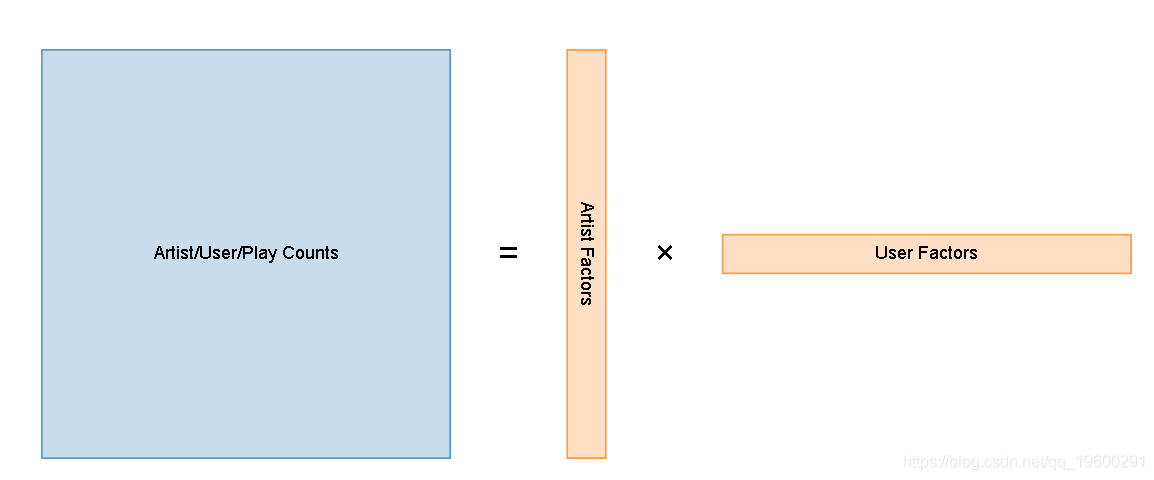
Artist/User/Play CountsArtist FactorsUser Factors=×

代替将每一个艺术家表示为全部360,000个可能用户的游戏计数的稀疏向量，在对矩阵进行因式分解以后，每一个艺术家将由50维密集向量表示。

经过减小这样的数据的维数，咱们实际上将输入矩阵压缩为两个小得多的矩阵。

潜在语义分析

出于本文的目的，咱们只须要知道SVD生成输入矩阵的低秩近似。

像这样使用SVD称为潜在语义分析（LSA）。全部真正涉及的是在这个分解空间中经过余弦距离得到最相关的艺术家：

class TopRelated(object): def __init__(self, artist_factors): # fully normalize artist_factors, so can compare with only the dot product norms = numpy.linalg.norm(artist_factors, axis=-1) self.factors = artist_factors / norms[:, numpy.newaxis] def get_related(self, artistid, N=10): scores = self.factors.dot(self.factors[artistid]) best = numpy.argpartition(scores, -N)[-N:] return sorted(zip(best, scores[best]), key=lambda x: -x[1])

潜在语义分析之因此得名，是由于在对矩阵进行分解以后，能够输入数据中潜在的隐藏结构 - 这能够被认为是揭示输入数据的语义。

​

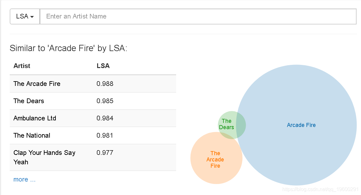
LSA 

相似于LSA的'Arcade Fire'：

​

 虽然LSA成功地归纳了咱们数据的某些方面，但这里的结果并非那么好。 

隐含的交替最小二乘法

已发现这些模型在推荐项目时效果很好，而且能够很容易地重复用于计算相关艺术家。

推荐系统中使用的许多MF模型都采用了明确的数据，用户使用相似5星级评定标准评估了他们喜欢和不喜欢的内容。

第一个挑战是有效地进行这种因式分解：经过将未知数视为负数，天真的实现将查看输入矩阵中的每一个条目。因为此处的维度大约为360K乘300K - 总共有超过1000亿条目要考虑，而只有1700万非零条目。

第二个问题是咱们不能肯定没有听艺术家的用户实际上意味着他们不喜欢它。可能还有其余缘由致使艺术家没有被收听，特别是考虑到咱们在数据集中每一个用户只有最多50位艺术家。

 使用二元偏好的不一样置信水平来学习分解矩阵表示：看不见的项目被视为负面且置信度低，其中当前项目被视为正面更高的信心。

那么目标是经过最小化平方偏差损失函数的置信加权和来学习用户因子X u和艺术家因子Y i：

def alternating_least_squares(Cui, factors, regularization, iterations=20): users, items = Cui.shape

    X = np.random.rand(users, factors) * 0.01    Y = np.random.rand(items, factors) * 0.01    Ciu = Cui.T.tocsr()    for iteration in range(iterations):        least_squares(Cui, X, Y, regularization)        least_squares(Ciu, Y, X, regularization)    return X, Ydef least_squares(Cui, X, Y, regularization):    users, factors = X.shape

    YtY = Y.T.dot(Y)    for u in range(users):        # accumulate YtCuY + regularization * I in A        A = YtY + regularization * np.eye(factors)        # accumulate YtCuPu in b        b = np.zeros(factors)        for i, confidence in nonzeros(Cui, u):            factor = Y[i]            A += (confidence - 1) * np.outer(factor, factor)            b += confidence * factor

        # Xu = (YtCuY + regularization * I)^-1 (YtCuPu)        X[u] = np.linalg.solve(A, b)

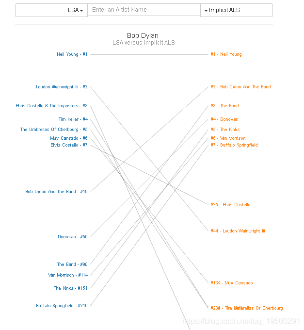
为了调用它，我使用与LSA中使用的置信矩阵相同的权重，而后以相同的方式计算相关的艺术家：

artist_factors ，user_factors = alternating_least_squares （bm25_weight （plays ），50 ）

与仅使用LSA相比，该方法能够产生明显更好的结果。 比较Bob Dylan的结果做为一个例子：